-
ABS
-
Computes absolute value of data-sets, Works only on real data-sets
(itype=0)
see also : MODULUS
REAL
-
ABSMAX
-
Absolute factor to which scale refers to for displaying and
plotting. Usually ABSMAX holds the largest point of the data-set,
but you can set it by hand in order to do absolute plots. ABSMAX is
recomputed whenever the data is changed.
You can force the ABSMAX to be recomputed by setting it to zero.
You can also hampers the recomputation of absmax (which can be VERY
long (on 3D for instance)) by setting it to a standard value at the
end of the command line
see also : MAX
SCALE
-
ADD
-
ADD name_of_file -or- ADDC name_of_file
permits to add to the current data-set the content of the file
name_of_file, which is in standard format. Works for both 1D, 2D and
3D data-sets.
see also : ADDDATA
ADDH
MULT
READ
-
ADDBASE
-
ADDBASE constant
Removes a constant to the data. The default value is the value of
SHIFT (computed by EVALN).
see also : EVALN
SHIFT
-
ADDC
-
Equivalent to ADD
see also : ADD
-
ADDDATA
-
Add the contents of the DATA buffer to the current data-set.
Equivalent to ADD but in-memory.
see also : ADD
ADDH
MAXDATA
MINDATA
MULT
MULTDATA
-
ADDH
-
ADDH name_of_file
Same as ADD, with H format files.
see also : ADD
ADDDATA
CONCAT
MULT
-
ADDNOISE
-
addnoise noise seed
add to the current data-set (1D, 2D, 3D) a white-gaussian,
characterized
by its level noise, and the random generator seed.
see also : EVALN
SIMU
SIMUN
-
aide
-
HELP (COMMAND)
Type help Name_of_item to get info about a specific command. H can
be used instead of HELP.
Use apropos topic, to find commands name related to a specific
topic.
Use help primer for a first introduction.
see also : apropos
-
ALERT
-
alert text
Creates a graphic alert box displaying the text. User must click in
the alert box to continue. Works only if the graphic mode has been
intialzed by isuing, at least once, a graphic command.
see also : ERROR
PRINT
-
ALGO
-
Context used to describe the current algorithm
Algo is a number of the form abc
where a, b and, c are the decimal digits.
c: 0 Gull and Daniel equation for Entropy
1 GIFA equation for Entropy
2 steepest descent equation is used
3 conjugate gradient is used
b: 0 single step iteration
1 line-maximization using parabolic fit.
2 : line-maximization using bracketing before parabolic
fit.
a: 0 no Wu correction
1 Wu correction is applied.
see also : conjg
gad
gifa
MAXENT
-
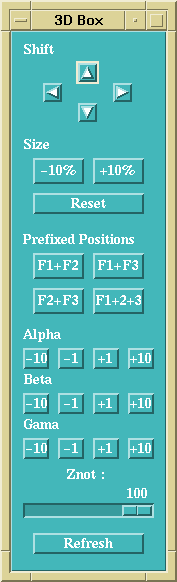
ALPHA
-
alpha a
This context is the angle along the OZ axis by which the cube is
rotated during a 3D display with the DISP3D/REF3D set of commands
see also : BETA
DISP3D
GAMA
-
APPLY
-
APPLY what_to_apply
Apply a windowing function to the data-set.
You can apply :
FILTER : applies the filter used during MaxEnt iterations, depends
on LB, GB, JCONS, FILTER
WINDOW : applies the window used during MaxEnt iterations.
see also : FILTER
GB
GET
JCONS
LB
PUT
SHOW
WINDOW
-
APPROX
-
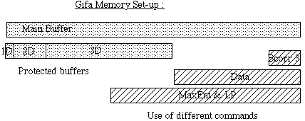
Used in the BCORR 3 module, to choose the way the baseline is
estimated.
0 : with ITERMA2 times a moving average filtering on a window of
size WINMA2.
1 : with a Legendre polynomial approximation of degree DEGRE.
+10 : with a linear interpolation of signal before approximation.
+100 : with an 'elastic effect' that is a rude way to prevent
from burying the weak lines.
see also : BCORR
BCORRP?
-
apropos
-
apropos topic
for GIFA on_line help
Search the string "topic" in all the help files available
see also : HELP
-
apsl
-
automatic 1D phase correction
APSL method
A.Heuer J.Magn.Reson. 91 p241 (1991)
uses the data buffer
you may want to adapt :
s_wdth : ration of line width to spectral width used for computing phases
p_wdth : ration of line width to spectral width used for broadening for peak picking
npk : minimum number of peaks needed for phasing
nfrst : the number of peaks used for first approx
see also : apsl_cp
PH
PHASE
-
apsl_cp
-
apsl_cp i sz
computes the phase of the peak centered on i, using +/-sz points
the phase of the peak is returned as a global variable called $returned
between -180 and 180
i has to be odd !
used as a routine by the macro apsl
see also : apsl
-
AR->DT
-
AR->DT size n
Extend the data-set up to size points long by predicting the missing
data points, using linear prediction.
n = 1 : following points predicted -> forward prediction
n = 2 : previous points predicted -> backward prediction
see also : BURG
DT->AR
ORDER
SVD->AR
-
AR->RT
-
AR->RT n
Solve the prediction-error polynomial, calculated from the
autoregressive coefficients. This is the third step of the LP-SVD
method.
n = 1 : forward coefficients are used to extracted forward roots
n = 2 : backward coefficients are used to extracted backward roots
n = 3 : both set of roots are computed
see also : AR->RT2
ARLIST
ORDER
RT->AR
SVD->AR
-
AR->RT2
-
AR->RT2 n
Equivalent to AR->RT, but seems to be more stable for very large
polynomial.
see also : ARLIST
ORDER
RT->AR
SVD->AR
-
AR->SP
-
Calculate the modulus of spectrum from the autoregressive Burg
coefficients. This is the so-called Burg spectrum, (sometimes
unfortunately called mem spectrum). The spectrum is computed to the
size of the current 1D buffer size.
see also : DT->AR
ORDER
-
ARLIST
-
ARLIST n i j
list the autoregressive coefficients from entry i to entry j.
n = 1 : forward coefficients
n = 2 : backward coefficients
see also : AR->DT
AR->RT
RT->AR
-
AXIS3D
-
axis3d fx where x is 1, 2, 3, 12, 13, or 123
This context holds the focal length that will be used for computing
a 3D display with the DISP3D/REF3D set of commands
see also : CHECK3D
DISP3D
REF3D

